This is a tutorial on decision trees as a classifier. I'll start with a top level discussion, thoroughly walk through an example, then cover a bit of the background math.
Decision trees as a classifier search for a series of rules that intelligently organize the given dataset. As a thought experiment, say you wanted to figure out what country a person is living in. First, you ask if they are in the east or west hemisphere. The answer is west. Are they within the continent of North America? Yes. Are they above or below the 42nd parallel? Above. At this point, you are fairly convinced the person is in Canada. You're not sure. It may be someone from the USA, but most of the people in the world that fit that criteria live in Canada.
Each question eliminates some of the ambiguity around what country a person is from. The better the question, the more ambiguity is removed. In this way, the decision tree automates the selection of sequences of questions to form good guesses about the class a sample is in. To demonstrate this, we'll use a common dataset and explore further what the decision tree is doing.
Introducing: Fisher's Iris Dataset
R. A. Fisher published The use of multiple measurements in taxonomic problems in 1936 which included the dataset we'll be using. This iris dataset is used time and time again across the literature, so it's a good dataset to be familiar with. More importantly, it makes for a very clean classification problem from four continuous variables. That is, each sample is labeled as one of three specific species of iris along with that sample's sepal and petal length and widths.
The full dataset has 150 samples, with an even split of 50 samples from each class where a class is a specific type of iris. The species names are 'setosa', 'versicolor', 'virginica'. Here is an excerpt from the data:
| Sepal Length (cm) | Sepal Width (cm) | Petal Length (cm ) | Petal Width (cm) | Iris Species | 5.1 | 3.5 | 1.4 | 0.2 | 0 |
| 5.7 | 4.4 | 1.5 | 0.4 | 0 |
| 5. | 2. | 3.5 | 1. | 1 |
| 6.6 | 3. | 4.4 | 1.4 | 1 |
| 7.6 | 3. | 6.6 | 2.1 | 2 |
| 6.9 | 3.2 | 5.7 | 2.3 | 2 |
Unfortunately, our three-dimensional vision mapped onto this two-dimensional medium constrains us to not directly plotting a four-dimensional dataset. One thing we can do instead is to plot the dataset in two dimensions for every possible pair of dimensions that exist as seen in this scatterplot:
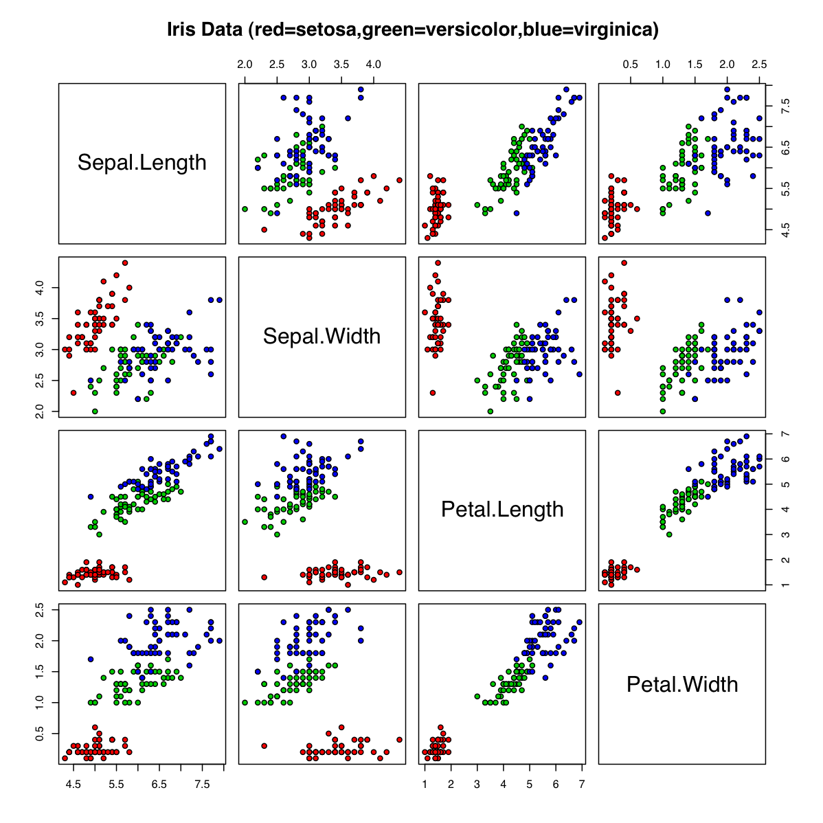
The red, green, and blue dots represent the species setosa, versicolor, and virginica respectively. The four dimensions of the dataset are labeled across the diagonal. For example, looking at the plot in the bottom row, third from the left, you'll see a plot comparing petal length with petal width. Intuitively, you'll see that the red 'blob' of dots is distinct from the other two species. The green and blue 'blob's have some overlap, but are also mostly distinct. Assuming all the flowers in this study were unbiased in growing conditions, sunlight, time to grow, and the like, this 'petal length vs petal width' graph makes a pretty clear point: The proportion of petal with and height stays roughly the same for all three species of iris, though the petal size differs greatly and consistently across all three species. Similar deductions can be drawn from most of the other graphs.
Decision Trees, By Example
Decision trees attempt to do with information theory what we did with our eyes in the last section. One variable at a time, decision trees try to draw boundaries between sections of data. Each drawn boundary acts as a 'decision' in the classification of different examples.
A Single Decision
In this section, I used sklearn and graphviz to make all the following visualizations. I'll supply one snippet to let the curious generate the trees as we go, but feel free to refer to the complete code I used to workshop this material in this ipython notebook. For those that don't want to code along, feel free to skip the snippet - the rest of the post will still be equally relevant.
In this snippet, a tree of depth=1 is generated, trained on the iris dataset, and saved as a graphviz dot file.
from sklearn.tree import DecisionTreeClassifier
from sklearn import tree
from sklearn import datasets

iris = datasets.load_iris()

clf = DecisionTreeClassifier(max_depth=1,criterion="entropy") # construct a decision tree.
clf.fit(iris.data,iris.target)  # train it on the dataset

dot_file = tree.export_graphviz(clf.tree_, out_file='tree_d1.dot', feature_names=iris.feature_names)  #export the tree to .dot file
dot_file.close() #close that dot file.
The resulting tree, as compiled by Graphviz using the command dot -T png tree_d1.dot -o tree_d1.png, is seen here:
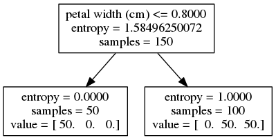
This image needs a bit of explanation. The top node represents the whole dataset. The whole dataset has 150 samples, as seen in the third line of that first node. We'll explain entropy more later, but for now, think of it as a formalization of the amount of uncertainty in the data. The first line on the top node gives us the decision our tree magically found. When that decision "petal width is less than or equal to 0.80 cm" is true for a given sample, that sample is assigned to the bottom left node. When it is false, the sample is assigned to the bottom right node.
On these two leaf nodes, the number of samples is shown on the second line. The number of samples broken down by class is on the third line. On the left leaf node, all 50 of the samples in class 1 and none from the other two classes are represented. Given the decision and the data at hand, we are certain to have a sample in class 1 (setosa). Since we are totally certain about that, uncertainty (entropy) is 0.
When our petal width <= 0.80 decider is false, the given sample is assigned to the right node. It works out that all 50 samples from class 2 (versicolor) and all 50 samples from class 3 (virginica) are assigned to this right leaf. Thus, when we're at this leaf given the decision, we're evenly unsure whether we're in class 2 or class 3. The amount of uncertainty this works out to be is 1.0. Again, we'll explain the math and meaning behind that later.
That's the explanation of the above tree, but what's really going on here? The tree chose to use the dimension petal length to make it's decision and the value 2.45 as it's decision level. Let's look at a histogram of the plot across that dimension:
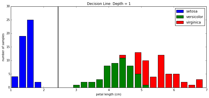
Above, you see the three classes represented as a histogram. The decision boundary is drawn at petal length = 2.45 cm as a vertical black line. As said in the decision tree's printout, you see here graphically that, indeed, all 50 of class 1 is to the left of the decision boundary and all of other 100 samples are to the right of the boundary.
Again, With a Second Layer
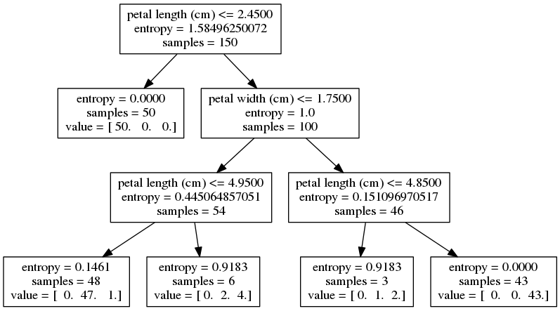
The previous snippet is re-used, but this time with depth=2. The resulting tree follows:
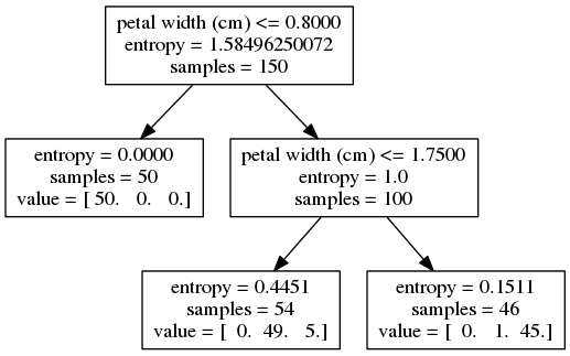
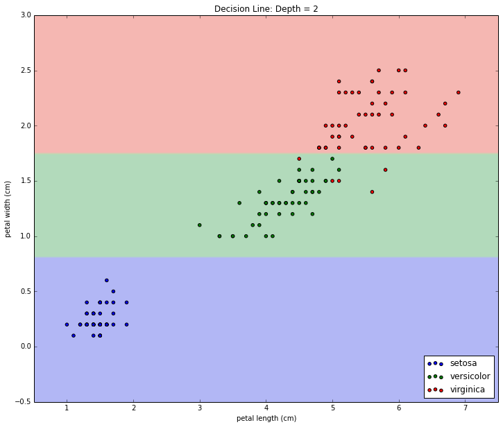
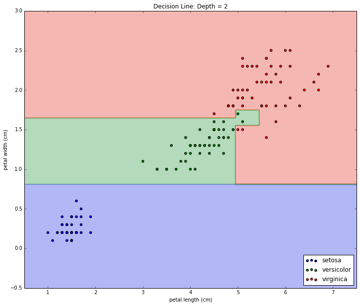
The left leaf at depth = 1 didn't split out into any more leaves because certainty has been achieved. The right leaf at depth = 1, however, did pick a new decision boundary at petal width <= 1.75 cm. This old leaf node forming a new decision makes two new leaf nodes. We see that the new decision does a good job splitting the classes, but unlike last time, the split is not perfect. Note that each of the bottom two leaf nodes' entropy, while small, is still greater than 0 and less than the preceding node's entropy = 1. Now that we're in two dimensions, let's visualize the boundary with a scatter plot (inspired by this example):
Again, With a Third Layer
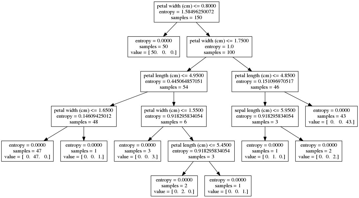
Same deal as last time. The tree is regenerated; this time with depth = 3. Here's the resulting tree:
And here's the visualized decision boundary:
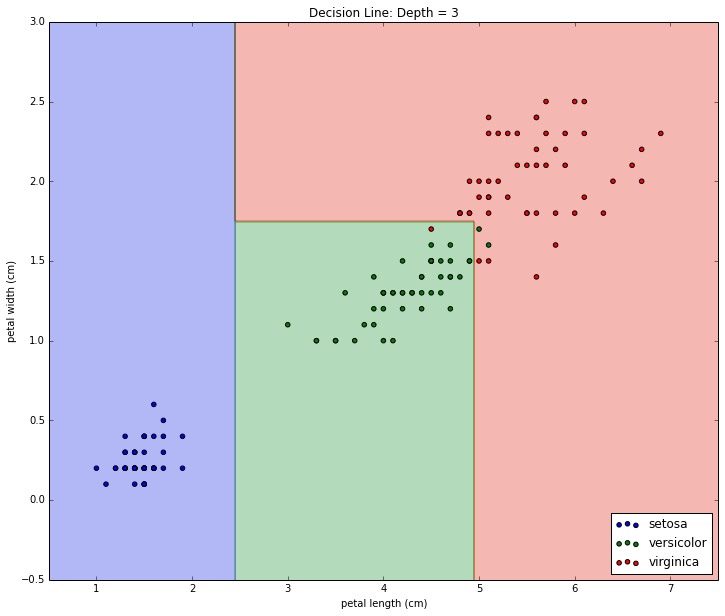
We're starting to get into statistically questionable territory here. While the decision boundary graph does look more intuitive to me, it's being made by adding decisions that only split off a handful of samples.
Growing Too Big
Let's discuss overfitting. Rebuilding the tree while totally unconstraining the depth will give you this hideous mass of a branches and leaves:
Petal length and width are still found at the top. Yes, we would be justified in using decision trees for variable selection and, if we do so here, could make a strong case that the petal dimensions are more important than the sepal dimensions.
Sepal length and width finally start being used, which tells us there is a chance they are also useful in terms of classifying samples. Yet there is a chance they are not useful and the tree may be 'learning' the noise in the data rather than any generally acceptable pattern. Volumes can be written on the math behind statistical significance applied to model building, but we'll keep this example visual and save further discussion for another post.
I re-train a tree with unconstrained depth on just the petal length and width (forcing it to ignore the sepal dimensions) so I can intuitively graph the decision boundary in two dimensions. Here is the resulting boundary:
Note the boundary looks to be the same as the depth = 3 boundary with one exception: There is an extra small green section (for class 2) carved out of the red (class 3) section around petal length = 5 cm and petal width = 1.6 cm. Intuitively, does that make sense to you? To me, it looks like that small extra section should belong to class 3, but the data just happen to have a few samples from class 2 that the algorithm 'memorized'.
There are plenty of ways to constrain tree growth: enforcing statistical significance at each decision, setting minimum number of samples per leaf, constraining the depth, etc. I won't discuss it further here, but I wanted to take this example to the end while demonstrating that overfitting does certainly need to be addressed when growing decision trees in the wild.
Entropy
Entropy is the quantification of uncertainty in data. With a coin flip, certainty is knowing on what side it will land before you flip it. In a game of poker, certainty is knowing the result of the next draw. In the case of how we framed the iris dataset, certainty is knowing what species of iris a given sample is just by looking at its sepal and petal dimensions.
The more uncertain, the higher the entropy. You are least certain of the outcome of a coin flip when the coin is fair. You starting gaining more certainty of what the next card will be in a poker game if you see other cards already dealt. Knowing nothing about the dimensions of the iris' sepal or petal, we are totally uncertain what species we're looking at. The graph we'll use to illustrate this is that same graph you'll see in every probability text book:
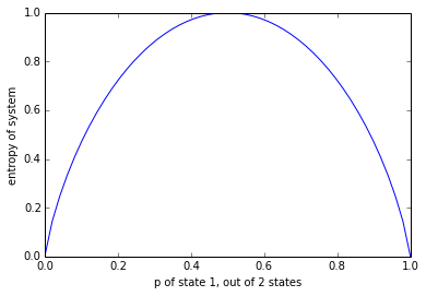
Along the x-axis, you'll find the probability of one state in a two state system (think of a coin flip - heads and tails). Along the y-axis, you'll find entropy. If the probability of heads is 50%, then the probability of tails is 50% and you have a fair coin. 'Fair' is to say we are totally uncertain of the result of the next coin flip, making this point the point with the highest entropy. The rest of the graph is symmetrical around this point. If heads has a 40% chance, then tails has a 60% chance. If heads has a 60% chance, then tails has a 40% chance. The entropy calculation doesn't care what label we apply to each state; only that there is a state with 40% likeliness and a state with 60% likeliness. The more biased a coin flip, the further from 50% the two states will be, and the closer to 0 our uncertainty (entropy) is.
Decision Evaluation
The same rules apply for decision trees with the three-state iris dataset. At any given leaf, the more biased the contained sample is, the less entropy it will have. Looking at the result of the decision in our depth=1 decision tree, we'll see two subsets of data. In the left leaf, you'll see entropy is now 0.0 because we are certain to have an iris of the first species. In the right leaf, entropy is 1.0 because we have an even choice between two classes (which works out to be the same as a unbiased coin flip). The total entropy post-choice is the left leaf's 0.0 plus the right leaf's 1.0 giving a total of 1.0. Compared to the original dataset's 1.58, the first decision results in a drop in entropy of 0.58.
Decision Selection
Let's use what we know now about entropy to see how the decision tree algorithm chooses its boundaries. The algorithm wants to pick the next decision that brings the most order to the dataset. We can search for this by calculating the total entropy that results for each possible decision.
In the same way we just evaluated the chosen decision boundary, let's evaluate every possible decision boundary for petal length and graph the result.
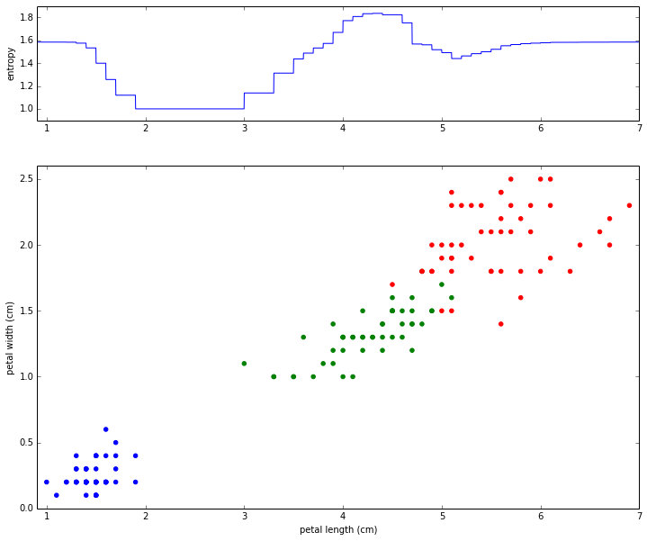
In the bottom graph, we see the scatterplot like before. In the upper graph, we see the total entropy that would result from drawing the decision boundary at the given petal length. Note how both graph are aligned and sharing the same x-axis. Drawing a decision at 4 cm will result in an entropy of 1.7 as seen at the same place in the upper graph. We now see that choosing a decision boundary somewhere within 1.9 and 3.0 results in the lowest possible amount of entropy, which is precisely what the algorithm did.
In practice, the algorithm has to search across all possible decision boundaries across all available variables. On this dataset, it works out that petal length and petal width both have decision boundaries that can result in our minimum entropy of 1.0, but the algorithm arbitrarily chose petal length in our example.
In summary: The decision tree grows sequences of choices to categorize data where each choice is made to minimize entropy in the resulting data.